Introduction
The goal of this project is to classify sonar signals as either rocks or mines using a neural network.
This webpage provides an overview of the dataset, preprocessing steps, model architecture, training, and evaluation results.
Data Preprocessing
The dataset consists of 60 numerical features and labels ('Rock' or 'Mine'). Below are the first few rows of the dataset:
| Feature_1 | Feature_2 | ... | Label |
|---|---|---|---|
| 0.02 | 0.03 | ... | Rock |
| 0.15 | 0.22 | ... | Mine |
Data Visualization
A 3-dimenisonal version of the 60-dimensional data is shown using Princple Component Analysis, a technique used to reduce dimensionality.

This shows the complex data set in 3 dimensions. One can see that there is no clear pattern that makes for easy classification, which makes this a good challenge for a neural network.
Model Overview
The neural network is composed of an input layer, a hidden layer with 32 nodes, and an output layer. Below is a diagram of the architecture:
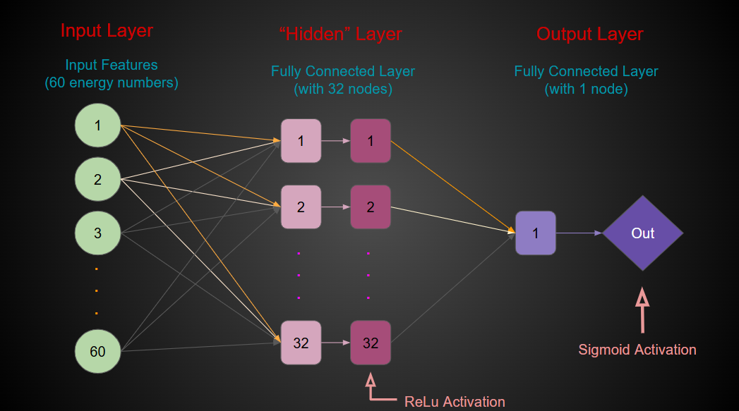
Inside the hidden layer, the darker colored boxes represent the activation function used, which is the Rectified Linear Unit (ReLU) function.
The output layer uses the Sigmoid activation function to produce a probability value between 0 and 1.
An activation function takes in a value and non-linearly transforms it to a desired range, usually between [-1, 1] or 0 and 1.
Neural Networks work by combining connections between nodes, where each connection has a weight associated with it.
After running cycles of training (epochs), the model learns to make accurate predictions by adjusting the weights to minimize the loss function.
This, combined with the nonlinearlity of activation functions, are what make neural networks so powerful.
Training and Loss Curves
The model was trained for 50 epochs, with loss curves for training and test datasets shown below:
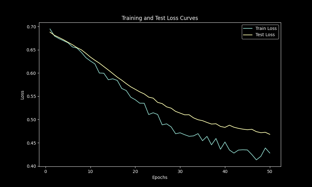
The model steadily gets better overtime, but doesn't overfit the training data.
Evaluation
The confusion matrix and classification report provide insights into model performance:
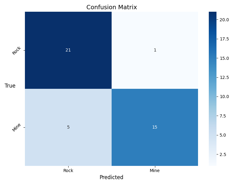
The confusion matrix can be hard to understand at first glance, but the idea is simple.
Looking at the top right box (white), this cell tells us that the model thought 1 object was a mine when it was actually a rock.
The bottom right box (normal blue) tells us that the model correctly predicted 15 objects that were mines as mines.
Similarily, the top left box (dark blue) tells us that the model correctly predicted 21 objects that were rocks as rocks.
The bottom left box (very light blue) tells us that the model thought 5 objects were rocks when they actually were mines.
Classification Report:
                    Precision  Recall  F1-Score  Support
            Rock      0.95    0.90      0.93      50
            Mine      0.92    0.96      0.94      50
The classification report is a more human-readable version of the confusion matrix.
It provides metrics such as precision, recall, and F1-score for each class.
Precision is the ratio of correctly predicted positive observations to the total predicted positives.
Recall is the ratio of correctly predicted positive observations to all actual positives.
F1-score is the weighted average of precision and recall.
Conclusion
This project aimed to educate the general audience about neural networks for (binary) classification while demonstrating the effectiveness of a simple neural network in classifying sonar signals.
As is shown through the training loss graph, the model steadily improves over time, and the confusion matrix and classification report show that the model performs well on the test data.
This means that the model is able to generalize well to unseen data, which is a key goal in machine learning.
Future work could involve exploring more advanced models, more advanced tasks, or additional feature engineering.